Model Evaluation – Machine Learning with Python

Evaluation Is Not a Decoration

A model is not useful because it produces predictions.

It is useful if:

it generalizes to new data
its errors are acceptable in context
the evaluation matches the real decision goal

This lesson focuses on disciplined evaluation for classification models.

Load Data

import pandas as pd

df = pd.read_csv("data/ml-ready/cdi-customer-churn.csv")

X = df.drop(columns="churn")
y = df["churn"]

Train/Test Split

from sklearn.model_selection import train_test_split

X_train, X_test, y_train, y_test = train_test_split(
    X,
    y,
    test_size=0.2,
    random_state=42,
    stratify=y
)

Define Preprocessing

from sklearn.compose import ColumnTransformer
from sklearn.preprocessing import OneHotEncoder, StandardScaler
from sklearn.pipeline import Pipeline

numeric_features = X.select_dtypes(include=["int64", "float64"]).columns
categorical_features = X.select_dtypes(include=["object"]).columns

numeric_transformer = Pipeline(
    steps=[("scaler", StandardScaler())]
)

categorical_transformer = Pipeline(
    steps=[("encoder", OneHotEncoder(handle_unknown="ignore"))]
)

preprocessor = ColumnTransformer(
    transformers=[
        ("num", numeric_transformer, numeric_features),
        ("cat", categorical_transformer, categorical_features)
    ]
)

Train a Baseline Classifier

from sklearn.linear_model import LogisticRegression

clf = Pipeline(
    steps=[
        ("preprocessor", preprocessor),
        ("classifier", LogisticRegression(max_iter=1000))
    ]
)

clf.fit(X_train, y_train)

Pipeline(steps=[('preprocessor',
                 ColumnTransformer(transformers=[('num',
                                                  Pipeline(steps=[('scaler',
                                                                   StandardScaler())]),
                                                  Index(['tenure_months', 'monthly_spend', 'support_calls'], dtype='str')),
                                                 ('cat',
                                                  Pipeline(steps=[('encoder',
                                                                   OneHotEncoder(handle_unknown='ignore'))]),
                                                  Index(['customer_id', 'contract_type', 'autopay'], dtype='str'))])),
                ('classifier', LogisticRegression(max_iter=1000))])

In a Jupyter environment, please rerun this cell to show the HTML representation or trust the notebook.
On GitHub, the HTML representation is unable to render, please try loading this page with nbviewer.org.

Predictions and Probabilities

import numpy as np

y_pred = clf.predict(X_test)
y_prob = clf.predict_proba(X_test)[:, 1]

y_pred[:10], np.round(y_prob[:10], 3)

(array([0, 1, 1, 1, 1, 1, 1, 1, 0, 1]),
 array([0.345, 0.666, 0.649, 0.827, 0.811, 0.825, 0.768, 0.57 , 0.411,
        0.666]))

Confusion Matrix

A confusion matrix breaks predictions into four counts:

True positives (TP)
False positives (FP)
True negatives (TN)
False negatives (FN)

from sklearn.metrics import confusion_matrix

cm = confusion_matrix(y_test, y_pred)
cm

array([[19, 39],
       [19, 83]])

cm_df = pd.DataFrame(
    cm,
    index=["Actual 0", "Actual 1"],
    columns=["Pred 0", "Pred 1"]
)

cm_df

	Pred 0	Pred 1
Actual 0	19	39
Actual 1	19	83

Accuracy Can Be Misleading

Accuracy answers:

How often was the prediction correct?

Accuracy can be misleading when:

classes are imbalanced
false positives and false negatives have different costs

For churn, missing a true churner (false negative) can be more costly than contacting a customer who would not churn (false positive).

Precision, Recall, and F1

from sklearn.metrics import accuracy_score, precision_score, recall_score, f1_score

accuracy = accuracy_score(y_test, y_pred)
precision = precision_score(y_test, y_pred)
recall = recall_score(y_test, y_pred)
f1 = f1_score(y_test, y_pred)

accuracy, precision, recall, f1

(0.6375, 0.680327868852459, 0.8137254901960784, 0.7410714285714286)

Interpretation:

Precision: among predicted churners, how many truly churned?
Recall: among true churners, how many did we catch?
F1: balance between precision and recall

Classification Report

A classification report summarizes key metrics per class.

from sklearn.metrics import classification_report

print(classification_report(y_test, y_pred, digits=3))

              precision    recall  f1-score   support

           0      0.500     0.328     0.396        58
           1      0.680     0.814     0.741       102

    accuracy                          0.637       160
   macro avg      0.590     0.571     0.568       160
weighted avg      0.615     0.637     0.616       160

Thresholds Change Behavior

By default, class predictions use a threshold of 0.5.

Lower thresholds often increase recall.
Higher thresholds often increase precision.

def predict_with_threshold(probs, threshold=0.5):
    return (probs >= threshold).astype(int)

thresholds = [0.3, 0.5, 0.7]

rows = []
for t in thresholds:
    y_t = predict_with_threshold(y_prob, threshold=t)
    rows.append({
        "threshold": t,
        "precision": precision_score(y_test, y_t),
        "recall": recall_score(y_test, y_t),
        "f1": f1_score(y_test, y_t)
    })

pd.DataFrame(rows)

	threshold	precision	recall	f1
0	0.3	0.647059	0.970588	0.776471
1	0.5	0.680328	0.813725	0.741071
2	0.7	0.786885	0.470588	0.588957

ROC Curve and AUC

The ROC curve shows performance across thresholds.

import matplotlib.pyplot as plt
from sklearn.metrics import roc_curve, roc_auc_score

fpr, tpr, thr = roc_curve(y_test, y_prob)
auc = roc_auc_score(y_test, y_prob)

auc

0.6511156186612576

fig, ax = plt.subplots()
ax.plot(fpr, tpr)
ax.set_xlabel("False Positive Rate")
ax.set_ylabel("True Positive Rate")
ax.set_title("ROC Curve")
plt.show()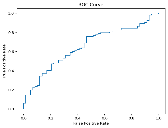

AUC ranges from 0.5 (no skill) to 1.0 (perfect separation).

Precision–Recall Curve

When the positive class is rare, ROC curves can look optimistic.

Precision–Recall curves focus directly on:

precision
recall

from sklearn.metrics import precision_recall_curve, average_precision_score

p, r, t = precision_recall_curve(y_test, y_prob)
ap = average_precision_score(y_test, y_prob)

ap

0.776966011701467

fig, ax = plt.subplots()
ax.plot(r, p)
ax.set_xlabel("Recall")
ax.set_ylabel("Precision")
ax.set_title("Precision–Recall Curve")
plt.show()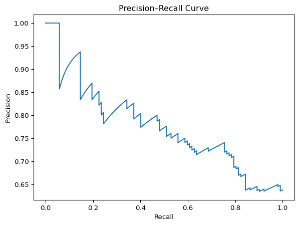

Average precision summarizes the PR curve in a single number.

Cross-Validation

A single train/test split can be noisy.

Cross-validation provides a more stable estimate of generalization.

from sklearn.model_selection import cross_val_score

scores = cross_val_score(clf, X, y, cv=5, scoring="f1")
scores, scores.mean()

(array([0.74782609, 0.75862069, 0.80869565, 0.74178404, 0.79475983]),
 np.float64(0.7703372583343606))

Looking Ahead

In the next lesson, we focus on overfitting and regularization.

The goal is not to chase metrics.

The goal is to build models that generalize.

	steps steps: list of tuples List of (name of step, estimator) tuples that are to be chained in sequential order. To be compatible with the scikit-learn API, all steps must define `fit`. All non-last steps must also define `transform`. See :ref:`Combining Estimators ` for more details.	[('preprocessor', ...), ('classifier', ...)]
	transform_input transform_input: list of str, default=None The names of the :term:`metadata` parameters that should be transformed by the pipeline before passing it to the step consuming it. This enables transforming some input arguments to ``fit`` (other than ``X``) to be transformed by the steps of the pipeline up to the step which requires them. Requirement is defined via :ref:`metadata routing `. For instance, this can be used to pass a validation set through the pipeline. You can only set this if metadata routing is enabled, which you can enable using ``sklearn.set_config(enable_metadata_routing=True)``. .. versionadded:: 1.6	None
	memory memory: str or object with the joblib.Memory interface, default=None Used to cache the fitted transformers of the pipeline. The last step will never be cached, even if it is a transformer. By default, no caching is performed. If a string is given, it is the path to the caching directory. Enabling caching triggers a clone of the transformers before fitting. Therefore, the transformer instance given to the pipeline cannot be inspected directly. Use the attribute ``named_steps`` or ``steps`` to inspect estimators within the pipeline. Caching the transformers is advantageous when fitting is time consuming. See :ref:`sphx_glr_auto_examples_neighbors_plot_caching_nearest_neighbors.py` for an example on how to enable caching.	None
	verbose verbose: bool, default=False If True, the time elapsed while fitting each step will be printed as it is completed.	False

	transformers transformers: list of tuples List of (name, transformer, columns) tuples specifying the transformer objects to be applied to subsets of the data. name : str Like in Pipeline and FeatureUnion, this allows the transformer and its parameters to be set using ``set_params`` and searched in grid search. transformer : {'drop', 'passthrough'} or estimator Estimator must support :term:`fit` and :term:`transform`. Special-cased strings 'drop' and 'passthrough' are accepted as well, to indicate to drop the columns or to pass them through untransformed, respectively. columns : str, array-like of str, int, array-like of int, array-like of bool, slice or callable Indexes the data on its second axis. Integers are interpreted as positional columns, while strings can reference DataFrame columns by name. A scalar string or int should be used where ``transformer`` expects X to be a 1d array-like (vector), otherwise a 2d array will be passed to the transformer. A callable is passed the input data `X` and can return any of the above. To select multiple columns by name or dtype, you can use :obj:`make_column_selector`.	[('num', ...), ('cat', ...)]
	remainder remainder: {'drop', 'passthrough'} or estimator, default='drop' By default, only the specified columns in `transformers` are transformed and combined in the output, and the non-specified columns are dropped. (default of ``'drop'``). By specifying ``remainder='passthrough'``, all remaining columns that were not specified in `transformers`, but present in the data passed to `fit` will be automatically passed through. This subset of columns is concatenated with the output of the transformers. For dataframes, extra columns not seen during `fit` will be excluded from the output of `transform`. By setting ``remainder`` to be an estimator, the remaining non-specified columns will use the ``remainder`` estimator. The estimator must support :term:`fit` and :term:`transform`. Note that using this feature requires that the DataFrame columns input at :term:`fit` and :term:`transform` have identical order.	'drop'
	sparse_threshold sparse_threshold: float, default=0.3 If the output of the different transformers contains sparse matrices, these will be stacked as a sparse matrix if the overall density is lower than this value. Use ``sparse_threshold=0`` to always return dense. When the transformed output consists of all dense data, the stacked result will be dense, and this keyword will be ignored.	0.3
	n_jobs n_jobs: int, default=None Number of jobs to run in parallel. ``None`` means 1 unless in a :obj:`joblib.parallel_backend` context. ``-1`` means using all processors. See :term:`Glossary ` for more details.	None
	transformer_weights transformer_weights: dict, default=None Multiplicative weights for features per transformer. The output of the transformer is multiplied by these weights. Keys are transformer names, values the weights.	None
	verbose verbose: bool, default=False If True, the time elapsed while fitting each transformer will be printed as it is completed.	False
	verbose_feature_names_out verbose_feature_names_out: bool, str or Callable[[str, str], str], default=True - If True, :meth:`ColumnTransformer.get_feature_names_out` will prefix all feature names with the name of the transformer that generated that feature. It is equivalent to setting `verbose_feature_names_out="{transformer_name}__{feature_name}"`. - If False, :meth:`ColumnTransformer.get_feature_names_out` will not prefix any feature names and will error if feature names are not unique. - If ``Callable[[str, str], str]``, :meth:`ColumnTransformer.get_feature_names_out` will rename all the features using the name of the transformer. The first argument of the callable is the transformer name and the second argument is the feature name. The returned string will be the new feature name. - If ``str``, it must be a string ready for formatting. The given string will be formatted using two field names: ``transformer_name`` and ``feature_name``. e.g. ``"{feature_name}__{transformer_name}"``. See :meth:`str.format` method from the standard library for more info. .. versionadded:: 1.0 .. versionchanged:: 1.6 `verbose_feature_names_out` can be a callable or a string to be formatted.	True
	force_int_remainder_cols force_int_remainder_cols: bool, default=False This parameter has no effect. .. note:: If you do not access the list of columns for the remainder columns in the `transformers_` fitted attribute, you do not need to set this parameter. .. versionadded:: 1.5 .. versionchanged:: 1.7 The default value for `force_int_remainder_cols` will change from `True` to `False` in version 1.7. .. deprecated:: 1.7 `force_int_remainder_cols` is deprecated and will be removed in 1.9.	'deprecated'

	categories categories: 'auto' or a list of array-like, default='auto' Categories (unique values) per feature: - 'auto' : Determine categories automatically from the training data. - list : ``categories[i]`` holds the categories expected in the ith column. The passed categories should not mix strings and numeric values within a single feature, and should be sorted in case of numeric values. The used categories can be found in the ``categories_`` attribute. .. versionadded:: 0.20	'auto'
	drop drop: {'first', 'if_binary'} or an array-like of shape (n_features,), default=None Specifies a methodology to use to drop one of the categories per feature. This is useful in situations where perfectly collinear features cause problems, such as when feeding the resulting data into an unregularized linear regression model. However, dropping one category breaks the symmetry of the original representation and can therefore induce a bias in downstream models, for instance for penalized linear classification or regression models. - None : retain all features (the default). - 'first' : drop the first category in each feature. If only one category is present, the feature will be dropped entirely. - 'if_binary' : drop the first category in each feature with two categories. Features with 1 or more than 2 categories are left intact. - array : ``drop[i]`` is the category in feature ``X[:, i]`` that should be dropped. When `max_categories` or `min_frequency` is configured to group infrequent categories, the dropping behavior is handled after the grouping. .. versionadded:: 0.21 The parameter `drop` was added in 0.21. .. versionchanged:: 0.23 The option `drop='if_binary'` was added in 0.23. .. versionchanged:: 1.1 Support for dropping infrequent categories.	None
	sparse_output sparse_output: bool, default=True When ``True``, it returns a :class:`scipy.sparse.csr_matrix`, i.e. a sparse matrix in "Compressed Sparse Row" (CSR) format. .. versionadded:: 1.2 `sparse` was renamed to `sparse_output`	True
	dtype dtype: number type, default=np.float64 Desired dtype of output.	<class 'numpy.float64'>
	handle_unknown handle_unknown: {'error', 'ignore', 'infrequent_if_exist', 'warn'}, default='error' Specifies the way unknown categories are handled during :meth:`transform`. - 'error' : Raise an error if an unknown category is present during transform. - 'ignore' : When an unknown category is encountered during transform, the resulting one-hot encoded columns for this feature will be all zeros. In the inverse transform, an unknown category will be denoted as None. - 'infrequent_if_exist' : When an unknown category is encountered during transform, the resulting one-hot encoded columns for this feature will map to the infrequent category if it exists. The infrequent category will be mapped to the last position in the encoding. During inverse transform, an unknown category will be mapped to the category denoted `'infrequent'` if it exists. If the `'infrequent'` category does not exist, then :meth:`transform` and :meth:`inverse_transform` will handle an unknown category as with `handle_unknown='ignore'`. Infrequent categories exist based on `min_frequency` and `max_categories`. Read more in the :ref:`User Guide `. - 'warn' : When an unknown category is encountered during transform a warning is issued, and the encoding then proceeds as described for `handle_unknown="infrequent_if_exist"`. .. versionchanged:: 1.1 `'infrequent_if_exist'` was added to automatically handle unknown categories and infrequent categories. .. versionadded:: 1.6 The option `"warn"` was added in 1.6.	'ignore'
	min_frequency min_frequency: int or float, default=None Specifies the minimum frequency below which a category will be considered infrequent. - If `int`, categories with a smaller cardinality will be considered infrequent. - If `float`, categories with a smaller cardinality than `min_frequency * n_samples` will be considered infrequent. .. versionadded:: 1.1 Read more in the :ref:`User Guide `.	None
	max_categories max_categories: int, default=None Specifies an upper limit to the number of output features for each input feature when considering infrequent categories. If there are infrequent categories, `max_categories` includes the category representing the infrequent categories along with the frequent categories. If `None`, there is no limit to the number of output features. .. versionadded:: 1.1 Read more in the :ref:`User Guide `.	None
	feature_name_combiner feature_name_combiner: "concat" or callable, default="concat" Callable with signature `def callable(input_feature, category)` that returns a string. This is used to create feature names to be returned by :meth:`get_feature_names_out`. `"concat"` concatenates encoded feature name and category with `feature + "_" + str(category)`.E.g. feature X with values 1, 6, 7 create feature names `X_1, X_6, X_7`. .. versionadded:: 1.3	'concat'

	penalty penalty: {'l1', 'l2', 'elasticnet', None}, default='l2' Specify the norm of the penalty: - `None`: no penalty is added; - `'l2'`: add a L2 penalty term and it is the default choice; - `'l1'`: add a L1 penalty term; - `'elasticnet'`: both L1 and L2 penalty terms are added. .. warning:: Some penalties may not work with some solvers. See the parameter `solver` below, to know the compatibility between the penalty and solver. .. versionadded:: 0.19 l1 penalty with SAGA solver (allowing 'multinomial' + L1) .. deprecated:: 1.8 `penalty` was deprecated in version 1.8 and will be removed in 1.10. Use `l1_ratio` instead. `l1_ratio=0` for `penalty='l2'`, `l1_ratio=1` for `penalty='l1'` and `l1_ratio` set to any float between 0 and 1 for `'penalty='elasticnet'`.	'deprecated'
	C C: float, default=1.0 Inverse of regularization strength; must be a positive float. Like in support vector machines, smaller values specify stronger regularization. `C=np.inf` results in unpenalized logistic regression. For a visual example on the effect of tuning the `C` parameter with an L1 penalty, see: :ref:`sphx_glr_auto_examples_linear_model_plot_logistic_path.py`.	1.0
	l1_ratio l1_ratio: float, default=0.0 The Elastic-Net mixing parameter, with `0 <= l1_ratio <= 1`. Setting `l1_ratio=1` gives a pure L1-penalty, setting `l1_ratio=0` a pure L2-penalty. Any value between 0 and 1 gives an Elastic-Net penalty of the form `l1_ratio * L1 + (1 - l1_ratio) * L2`. .. warning:: Certain values of `l1_ratio`, i.e. some penalties, may not work with some solvers. See the parameter `solver` below, to know the compatibility between the penalty and solver. .. versionchanged:: 1.8 Default value changed from None to 0.0. .. deprecated:: 1.8 `None` is deprecated and will be removed in version 1.10. Always use `l1_ratio` to specify the penalty type.	0.0
	dual dual: bool, default=False Dual (constrained) or primal (regularized, see also :ref:`this equation `) formulation. Dual formulation is only implemented for l2 penalty with liblinear solver. Prefer `dual=False` when n_samples > n_features.	False
	tol tol: float, default=1e-4 Tolerance for stopping criteria.	0.0001
	fit_intercept fit_intercept: bool, default=True Specifies if a constant (a.k.a. bias or intercept) should be added to the decision function.	True
	intercept_scaling intercept_scaling: float, default=1 Useful only when the solver `liblinear` is used and `self.fit_intercept` is set to `True`. In this case, `x` becomes `[x, self.intercept_scaling]`, i.e. a "synthetic" feature with constant value equal to `intercept_scaling` is appended to the instance vector. The intercept becomes ``intercept_scaling * synthetic_feature_weight``. .. note:: The synthetic feature weight is subject to L1 or L2 regularization as all other features. To lessen the effect of regularization on synthetic feature weight (and therefore on the intercept) `intercept_scaling` has to be increased.	1
	class_weight class_weight: dict or 'balanced', default=None Weights associated with classes in the form ``{class_label: weight}``. If not given, all classes are supposed to have weight one. The "balanced" mode uses the values of y to automatically adjust weights inversely proportional to class frequencies in the input data as ``n_samples / (n_classes * np.bincount(y))``. Note that these weights will be multiplied with sample_weight (passed through the fit method) if sample_weight is specified. .. versionadded:: 0.17 class_weight='balanced'	None
	random_state random_state: int, RandomState instance, default=None Used when ``solver`` == 'sag', 'saga' or 'liblinear' to shuffle the data. See :term:`Glossary ` for details.	None
	solver solver: {'lbfgs', 'liblinear', 'newton-cg', 'newton-cholesky', 'sag', 'saga'}, default='lbfgs' Algorithm to use in the optimization problem. Default is 'lbfgs'. To choose a solver, you might want to consider the following aspects: - 'lbfgs' is a good default solver because it works reasonably well for a wide class of problems. - For :term:`multiclass` problems (`n_classes >= 3`), all solvers except 'liblinear' minimize the full multinomial loss, 'liblinear' will raise an error. - 'newton-cholesky' is a good choice for `n_samples` >> `n_features * n_classes`, especially with one-hot encoded categorical features with rare categories. Be aware that the memory usage of this solver has a quadratic dependency on `n_features * n_classes` because it explicitly computes the full Hessian matrix. - For small datasets, 'liblinear' is a good choice, whereas 'sag' and 'saga' are faster for large ones; - 'liblinear' can only handle binary classification by default. To apply a one-versus-rest scheme for the multiclass setting one can wrap it with the :class:`~sklearn.multiclass.OneVsRestClassifier`. .. warning:: The choice of the algorithm depends on the penalty chosen (`l1_ratio=0` for L2-penalty, `l1_ratio=1` for L1-penalty and `0 < l1_ratio < 1` for Elastic-Net) and on (multinomial) multiclass support: ================= ======================== ====================== solver l1_ratio multinomial multiclass ================= ======================== ====================== 'lbfgs' l1_ratio=0 yes 'liblinear' l1_ratio=1 or l1_ratio=0 no 'newton-cg' l1_ratio=0 yes 'newton-cholesky' l1_ratio=0 yes 'sag' l1_ratio=0 yes 'saga' 0<=l1_ratio<=1 yes ================= ======================== ====================== .. note:: 'sag' and 'saga' fast convergence is only guaranteed on features with approximately the same scale. You can preprocess the data with a scaler from :mod:`sklearn.preprocessing`. .. seealso:: Refer to the :ref:`User Guide ` for more information regarding :class:`LogisticRegression` and more specifically the :ref:`Table ` summarizing solver/penalty supports. .. versionadded:: 0.17 Stochastic Average Gradient (SAG) descent solver. Multinomial support in version 0.18. .. versionadded:: 0.19 SAGA solver. .. versionchanged:: 0.22 The default solver changed from 'liblinear' to 'lbfgs' in 0.22. .. versionadded:: 1.2 newton-cholesky solver. Multinomial support in version 1.6.	'lbfgs'
	max_iter max_iter: int, default=100 Maximum number of iterations taken for the solvers to converge.	1000
	verbose verbose: int, default=0 For the liblinear and lbfgs solvers set verbose to any positive number for verbosity.	0
	warm_start warm_start: bool, default=False When set to True, reuse the solution of the previous call to fit as initialization, otherwise, just erase the previous solution. Useless for liblinear solver. See :term:`the Glossary `. .. versionadded:: 0.17 warm_start to support lbfgs, newton-cg, sag, saga solvers.	False
	n_jobs n_jobs: int, default=None Does not have any effect. .. deprecated:: 1.8 `n_jobs` is deprecated in version 1.8 and will be removed in 1.10.	None